Data Fitting with SciPy - Introduction to Scientific Python for Chemical and Materials Engineers

17.1Lesson goals¶

Perform a least squares fitting analysis using the scipy.optimize.curve_fit() function.
Report fitting parameters and standard errors / uncertainties.
Calculate the R² of a fit.
Combine NumPy, Matplotlib, and SciPy skills to analyze and display data.
Set a fit range and provide initial guesses to fitted parameters.
Include measurement uncertainty as weights in scipy.optimize.curve_fit().

17.2Overview¶

Analyzing measured data with a theoretical model is a common task for a scientist and engineer. We often model (i.e., “fit”) datasets with a mathematical function like lines, sinusoidal waves, or exponentials to extract out a metrics related to materials properties, processing conditions, or physical phenomena.

Least squares regression analysis is commonly used when fitting data, and you may have done this before with other software packages (e.g., Microsoft Excel’s LINEST function). This lesson will go over how to do basic least squares regression analysis using the SciPy library. We first will go over how to perform a regression analysis by fitting a line through a dataset and extract out both fitted values and standard errors on the fit. We will also show how you can calculate the $R^2$ value to quantitative asses the quality of your fit. We then will show you how you can perform non-linear fitting, include fit ranges and initial guesses to fitted parameters, and how include with error bars that represent measurement uncertainty to your fits.

17.3Installing the SciPy library¶

SciPy is not part of the standard Python library. However many library repositories have it. The steps below explain how to instally SciPy to your Python virtual environment using Miniforge:

Open up Miniforge.
Activate your Python environment.
Type in conda install -c conda-forge scipy.
Follow the onscreen commands to install the library.
Restart VSCode or JupyterLab if they are currently opened once the library is installed.

17.4Importing SciPy for data fitting¶

Since we are going to analyze and plot datasets, let’s load NumPy, Matplotlib’s pyplot module (matplotlib.pyplot), and the curve_fit() function from SciPy’s optimization module (scipy.optimize):

# Need NumPy and Matplotlib for basic plotting
import numpy as np
from matplotlib import pyplot as plt
from matplotlib import ticker as tck

# Load curve_fit() from the scipy.optimize library
from scipy.optimize import curve_fit

Let’s also set some plotting defaults for our session using rcParams:

# rcParams overrides

# Title size & color
plt.rcParams["axes.titlesize"] = 16

# Axis label size
plt.rcParams["axes.labelsize"] = 14

# x-axis values
plt.rcParams["xtick.labelsize"] = 12
plt.rcParams["xtick.direction"] = "in"
plt.rcParams["xtick.top"] = True

# y-axis values
plt.rcParams["ytick.labelsize"] = 12
plt.rcParams["ytick.direction"] = "in"
plt.rcParams["ytick.right"] = True

# Spines (the actual axis borders)
plt.rcParams["axes.spines.bottom"] = True
plt.rcParams["axes.spines.top"] = True
plt.rcParams["axes.spines.left"] = True
plt.rcParams["axes.spines.right"] = True

# Legend settings
plt.rcParams["legend.frameon"] = False
plt.rcParams["legend.fontsize"] = 14

17.5Linear fitting¶

Let’s start by fitting a simple dataset with a line. The example below is based on analyzing current-voltage data taken from of a resistor, which is a fundamental device in electrical circuits. A resistor’s electrical response follows Ohm’s law, which states that there is a linear relationship between the voltage across a resistor and the current passing through a resistor via the equation,

V = IR

(1)

where $V$ is the voltage across a resistor (units: volt, $\text{V}$ ), $I$ is the current passing through a resistor (units: amps, $\text{A}$ ), and $R$ is the inherent electrical “resistance” of the device (units: $\text{V}/\text{A} = \Omega$ ). In circuit analysis, electrical devices and materials are often modeled as resistors, so measuring the resistance is a common task for a scientist or engineer.

Data for this exercise can be found in the file iv-data.csv. This file has two columns of data: (1) the sourced current and (2) measured voltage of the measurement. The first row has the labels for each column and the second row has the units for each column. Since this is a CSV file, each column is separated with a , symbol. Let’s first see what the data looks like:

# -----------------------------------------------------------------------------
# Load data
# -----------------------------------------------------------------------------
iv_data = np.loadtxt("./static/example-data/iv-data.csv", delimiter=",", skiprows=2)

current = iv_data[:, 0]
voltage = iv_data[:, 1]

# -----------------------------------------------------------------------------
# Plot data
# -----------------------------------------------------------------------------

iv_fig = plt.figure()
iv_ax = iv_fig.add_subplot(1, 1, 1)

# Plot iv data
iv_ax.plot(current, voltage,
         label="measured data",
         marker="o",
         markersize=8,
         linestyle="none",
         color="blue")

iv_ax.set_title("Ohm's Law Analysis")
iv_ax.set_xlabel("I [A]")
iv_ax.set_ylabel("V [V]")
iv_ax.set_xlim(left=0, right=6.5E-3)
iv_ax.set_ylim(bottom=0, top=2.5)
iv_ax.xaxis.set_major_locator(tck.MultipleLocator(0.002))
iv_ax.xaxis.set_minor_locator(tck.AutoMinorLocator(2))
iv_ax.yaxis.set_minor_locator(tck.AutoMinorLocator(2))

plt.show()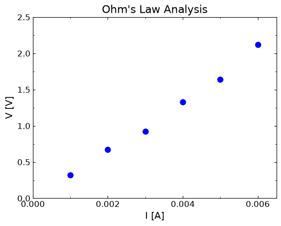

The dataset looks linear so we should expect a good line fit. We have stored the current values (the $x$ -axis data) in the variable current and the voltage values (the $y$ -axis data) in the variable voltage. The main function we are going to use is scipy.optimize.curve_fit(), which has three required arguments. The first positional argument is f, which is the function to fit (in our case a line). The second positional argument is xdata, which represents the $x$ -axis (i.e., independent variable) data. The third argument is ydata, which represents the $y$ -axis (i.e., dependent variable) data. There are more optional arguments (we will look at these arguments soon), but right now we need to create the function that will be assigned to f. Recall that a line can be represented as,

y = mx + b

(2)

where $y$ is the dependent variable, $x$ is independent variable, $m$ is slope of the line, and $b$ is $y$ -intercept (i.e., the $y$ value when $x = 0$ ). In terms of Python, we can write the following function to represent a line:

def linearFunc(x, intercept, slope):
    y = intercept + slope * x
    return y

Now let’s have scipy.optimize.curve_fit() to do the fit:

# Fit!
popt, pcov = curve_fit(linearFunc, current, voltage)

Our call of scipy.optimize.curve_fit() returns two variables: popt and pcov. According to the curve_fit()'s documentation, popt is a 1D array that contains the optimized fitted parameters. The position of the parameters in this array is based on the argument order in our function code block. For us, this means that the first value listed is the intercept and the second value listed is the slope. Let’s extract out these values from popt:

print("popt:")
print(popt)

# Values
intercept = popt[0]
slope = popt[1]

print(f"intercept: {intercept:.4f} V")
print(f"slope: {slope:.1f} ohm")

popt:
[-6.53333147e-02  3.51999996e+02]
intercept: -0.0653 V
slope: 352.0 ohm

The pcov variable is a 2D array that contains the estimated variances and covariances of the fitted parameters. For our needs, we will just look at the variances of the fitted variables, which reside on the diagonal of the array. Let’s extract these diagonal terms and take the square root of them as this will represent the standard fitting error (a.k.a., the standard uncertainty) of each parameter:

print("pcov:")
print(pcov)

# Errors -> Need to take the sqrt
intercept_err = np.sqrt(pcov[0][0])
slope_err = np.sqrt(pcov[1][1])

print(f"intercept std. error: {intercept_err:.4f} V")
print(f"slope std. error: {slope_err:.1f} ohm")

pcov:
[[ 3.38288914e-03 -7.80666739e-01]
 [-7.80666739e-01  2.23047639e+02]]
intercept std. error: 0.0582 V
slope std. error: 14.9 ohm

The code block above provides us with the basic fitting results. For completion, let’s make a plot that shows the optimized line with our data. The code below goes over all the necessary steps to make this happen:

# -----------------------------------------------------------------------------
# Plot data
# -----------------------------------------------------------------------------

iv_fig = plt.figure()
iv_ax = iv_fig.add_subplot(1, 1, 1)

# Plot iv data
iv_ax.plot(current, voltage,
         label="measured data",
         marker="o",
         markersize=8,
         linestyle="none",
         color="blue")

# Create fit line
yfit = intercept + slope * current

# Plot fit data
iv_ax.plot(current, yfit,
        color="red",
        label="fit",
        linestyle="dashed")

iv_ax.set_title("Ohm's Law Analysis")
iv_ax.set_xlabel("I [A]")
iv_ax.set_ylabel("V [V]")
iv_ax.set_xlim(left=0, right=6.5E-3)
iv_ax.set_ylim(bottom=0, top=2.5)
iv_ax.xaxis.set_major_locator(tck.MultipleLocator(0.002))
iv_ax.xaxis.set_minor_locator(tck.AutoMinorLocator(2))
iv_ax.yaxis.set_minor_locator(tck.AutoMinorLocator(2))
iv_ax.legend()

plt.show()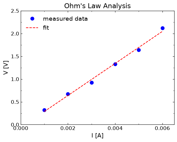

To create the fit line, we first create yfit, which is an array that stores calculated voltages using current (our $x$ -values) and intercept and slope (our fitting results). We then add this dataset to our previous plot. The code below consolidates all the previous steps into one easy to reference block:

# Linear fitting example
# -----------------------------------------------------------------------------
# Libraries
# -----------------------------------------------------------------------------
import numpy as np
from matplotlib import pyplot as plt
from scipy.optimize import curve_fit

# -----------------------------------------------------------------------------
# Load data
# -----------------------------------------------------------------------------
iv_data = np.loadtxt("./static/example-data/iv-data.csv", delimiter=",", skiprows=2)

current = iv_data[:, 0]
voltage = iv_data[:, 1]

# -----------------------------------------------------------------------------
# Least squares analysis
# -----------------------------------------------------------------------------

# Linear equation
def linearFunc(x, intercept, slope):
    y = intercept + slope * x
    return y

# Fit!
popt, pcov = curve_fit(linearFunc, current, voltage)

# Extract parameters
intercept = popt[0]
slope = popt[1]
intercept_err = np.sqrt(pcov[0][0])
slope_err = np.sqrt(pcov[1][1])

# -----------------------------------------------------------------------------
# Plot data
# -----------------------------------------------------------------------------

iv_fig = plt.figure()
iv_ax = iv_fig.add_subplot(1, 1, 1)

# Plot iv data
iv_ax.plot(current, voltage,
         label="measured data",
         marker="o",
         markersize=8,
         linestyle="none",
         color="blue")

# Create fit line
yfit = intercept + slope * current

# Plot fit data
iv_ax.plot(current, yfit,
        color="red",
        label="fit",
        linestyle="dashed")

iv_ax.set_title("Ohm's Law Analysis")
iv_ax.set_xlabel("I [A]")
iv_ax.set_ylabel("V [V]")
iv_ax.set_xlim(left=0, right=6.5E-3)
iv_ax.set_ylim(bottom=0, top=2.5)
iv_ax.xaxis.set_major_locator(tck.MultipleLocator(0.002))
iv_ax.xaxis.set_minor_locator(tck.AutoMinorLocator(2))
iv_ax.yaxis.set_minor_locator(tck.AutoMinorLocator(2))
iv_ax.legend()

plt.show()

# -----------------------------------------------------------------------------
# Display results
# -----------------------------------------------------------------------------
print(f"intercept: {intercept:.4f} V")
print(f"slope: {slope:.1f} ohm")
print(f"intercept std. error: {intercept_err:.4f} V")
print(f"slope std. error: {slope_err:.1f} ohm")

intercept: -0.0653 V
slope: 352.0 ohm
intercept std. error: 0.0582 V
slope std. error: 14.9 ohm

17.6 $R^2$ of fit¶

We can quantify how “good” our fit is using the “R squared” value (often denoted as $R^2$ , the coefficient of determination). Mathematically,

R^2 = 1 - \frac{SS_{res}}{SS_{tot}}

(3)

where $SS_{res}$ is called the “residual sum of squares” and $SS_{tot}$ is called the “total sum of squares”. Let’s first focus on the total sum of squares, $SS_{tot}$ , which is,

SS_{tot} = \sum_{i}^n (y_i - \bar{y})^2

(4)

where $y_i$ is the $i$ -th dependent variable in a dataset of size $n$ (in our case these are the individual voltage values), and $\bar{y}$ value is the average of all $y_i$ values. We define $\bar{y}$ as,

\bar{y} = \frac{1}{n} \sum_{i}^n y_i

(5)

Since our measured voltages (i.e., the $y_i$ values) are stored in the array voltage, let’s use the NumPy function numpy.mean() to calculate the average voltage (i.e., $\bar{y}$ ) and store it in the variable voltage_mean:

voltage_mean = np.mean(voltage)
print(f"voltage_mean: {voltage_mean:.3f} V")

voltage_mean: 1.167 V

Now let’s calculate $SS_{tot}$ . The code block below shows how to do this by first creating an intermediate array called deviation_squared that stores the square of the deviation between the voltage values and the average voltage. Then we use another useful NumPy function, numpy.sum(), to sum all the values in deviation_squared (also an array). Similar to numpy.mean(), we can have numpy.sum() sum up along particular axes of an array, but for our needs we need to sum up all values.

deviation_squared = (voltage - voltage_mean)**2
ss_tot = np.sum(deviation_squared)
print(f"ss_tot: {ss_tot:.3f} V^2")

ss_tot: 2.184 V^2

Now let’s define and calculate $SS_{res}$ (i.e., the other term we need in order to calculate $R^2$ ). Mathematically, $SS_{res}$ is defined as,

SS_{res} = \sum_{i}^n(y_i - f_i)^2

(6)

where $f_i$ represents the calculated $i$ -th dependent variable based on the fitting equation. For our situation, this is our yfit array in the main code block, which we use to create the fit line in the figure.

Let’s go ahead and calculate $SS_{res}$ for our example,

error_squared = (voltage - yfit)**2
ss_res = np.sum(error_squared)
print(f"ss_res: {ss_res:.3f} V^2")

ss_res: 0.016 V^2

We again use an intermediate variable, this time called error_squared, that stores the deviation between the measured voltages and the modeled voltage values from yfit. We then use the numpy.sum() function to sum up all the values in this array to get $SS_{res}$ .

With these two values, we can now calculate R²:

r_squared = 1 - ss_res / ss_tot
print(f"R squared: {r_squared:.4f}")

R squared: 0.9929

For reference, the code below combines all of these steps together into one single code block.

# Calculate voltage mean
voltage_mean = np.mean(voltage)
print(f"voltage_mean: {voltage_mean:.3f} V")

# Calculate total sum of squares, ss_tot
deviation_squared = (voltage - voltage_mean)**2
ss_tot = np.sum(deviation_squared)
print(f"ss_tot: {ss_tot:.3f} V^2")

# Calculate residual sum of squares, ss_res
error_squared = (voltage - yfit)**2
ss_res = np.sum(error_squared)
print(f"ss_res: {ss_res:.3f} V^2")

# Calculate R squared
r_squared = 1 - ss_res / ss_tot
print(f"R squared: {r_squared:.4f}")

voltage_mean: 1.167 V
ss_tot: 2.184 V^2
ss_res: 0.016 V^2
R squared: 0.9929

The $R^2$ value is a useful metric to calculate for any fit so let’s create a generalized, function-based version of our code so we can easily deploy in other code blocks:

def rsquared(y, yfit):
    """
    Calculate the R^2 value of a fit.

    Parameters
    ----------
    y : NumPy array (numpy.ndarray)
        Dependent variable values of dataset.

    y_fit : NumPy array (numpy.ndarray)
        Calculated dependent values based on fitted results.

    Returns
    -------
    r_squared : float
        The R^2 value of a fit.
    """

    # Calculate mean
    y_mean = np.mean(y)
    # Calculate total sum of squares, ss_tot
    deviation_squared = (y - y_mean)**2
    ss_tot = np.sum(deviation_squared)
    # Calculate residual sum of squares, ss_res
    error_squared = (y - yfit)**2
    ss_res = np.sum(error_squared)
    # Calculate R squared
    r_squared = 1 - ss_res / ss_tot
    return r_squared

We can now quickly calculate the $R^2$ value by issuing the commands:

# call R squared for V=IR analysis

r_squared = rsquared(voltage, yfit)
r_squared = round(r_squared, 4)
print("R^2:", r_squared)

R^2: 0.9929

17.7Non-linear curve fitting¶

We can also use scipy.optimize.curve_fit() to fit datasets that do not have a linear relationship. The overall process is really no different from linear fitting. We just need to create a non-linear function and account for the new variables in popt and pcov.

To see this in action, first download the CSV file magnetoresistance-data.csv, which contains a set of measured data points from a sample whose electrical resistance changes as function of magnetic field. This data will follow a second-order polynomial-like dependence (i.e., a parabola) that follows the functional form:

y = A + Bx + Cx^2

(8)

where $A$ is a constant, $B$ is the linear parameter, and $C$ is the second-order or “quadratic” term. The block of code below is the entire code needed to fully run this regression analysis:

# Non-linear fitting example
# -----------------------------------------------------------------------------

# -----------------------------------------------------------------------------
# Load data
# -----------------------------------------------------------------------------
iv_data = np.loadtxt("./static/example-data/magnetoresistance-data.csv",
                     delimiter=",",
                     skiprows=2)

magnetic_field = iv_data[:, 0]
resistance = iv_data[:, 1]

# -----------------------------------------------------------------------------
# Least squares analysis
# -----------------------------------------------------------------------------

# Parabola equation
def parabolaFunc(x, constant, linear, quadratic):
    """Parabola fitting function"""
    y = constant + linear * x + quadratic * (x**2)
    return y

# Fit!
popt, pcov = curve_fit(parabolaFunc, magnetic_field, resistance)

# Extract parameters
constant = popt[0]
linear = popt[1]
quadratic = popt[2]
constant_err = np.sqrt(pcov[0][0])
linear_err = np.sqrt(pcov[1][1])
quadratic_err = np.sqrt(pcov[2][2])

# Create fitted dataset
resistance_calc = (constant + (linear * magnetic_field)
                  + (quadratic * (magnetic_field**2)))

# R squared
r_squared = rsquared(resistance, resistance_calc)
r_squared = round(r_squared, 4)

# -----------------------------------------------------------------------------
# Plot data
# -----------------------------------------------------------------------------
mr_fig = plt.figure()
mr_fig = mr_fig.add_subplot(1, 1, 1)

# Plot iv data
mr_fig.plot(magnetic_field, resistance,
         label="measured data",
         marker="o",
         markersize=8,
         linestyle="none",
         color="blue")

# Plot fit data
mr_fig.plot(magnetic_field, resistance_calc,
        color="red",
        label="fit",
        linestyle="dashed")

mr_fig.set_title("Magnetoresistance analysis")
mr_fig.set_xlabel("B [T]")
mr_fig.set_ylabel("R [$\\Omega$]")
mr_fig.xaxis.set_minor_locator(tck.AutoMinorLocator(2))
mr_fig.yaxis.set_minor_locator(tck.AutoMinorLocator(2))
mr_fig.legend()


# -----------------------------------------------------------------------------
# Display plot & results
# -----------------------------------------------------------------------------
plt.show()

print(f"constant: {constant:.4f} ohm")
print(f"linear = {linear:.2E} ohm/T")
print(f"quadratic = {quadratic:.2E} ohm/T^2")
print(f"R squared: {r_squared:.4f}")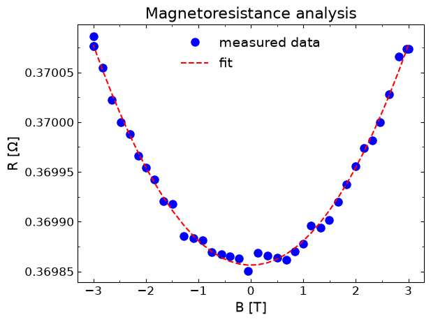

constant: 0.3699 ohm
linear = -1.19E-08 ohm/T
quadratic = 2.46E-05 ohm/T^2
R squared: 0.9946

There is no real structural difference in our code from the previous line fitting example. The only differences in the code are in replacing our linear function linearFunc() with the polynomial function parabolaFunc(), renaming the variables for the measured data, and adjusting the code to handle the new fitting parameters. In short, once you know how to perform the line fit, you can fit any other function!

17.8Other useful fitting options¶

17.8.1Fitting bounds¶

We can limit the range of data points we want to fit over by creating subarrays of the total data. The code block below demonstrates this using the magnetoresistance data from earlier:

# Non-linear fitting example w/ fitting bounds

# -----------------------------------------------------------------------------
# Load data
# -----------------------------------------------------------------------------
iv_data = np.loadtxt("./static/example-data/magnetoresistance-data.csv",
                     delimiter=",",
                     skiprows=2)

magnetic_field = iv_data[:, 0]
resistance = iv_data[:, 1]

# -----------------------------------------------------------------------------
# Data to fit over
# -----------------------------------------------------------------------------

# Data point number
min_index = 7
max_index = 40

# Sub arrays of data to fit over
magnetic_field_fit = magnetic_field[min_index: max_index]
resistance_fit = resistance[min_index: max_index]

# -----------------------------------------------------------------------------
# Least squares analysis
# -----------------------------------------------------------------------------

# Fit the subset!
popt, pcov = curve_fit(parabolaFunc, magnetic_field_fit, resistance_fit)

# Extract parameters
constant = popt[0]
linear = popt[1]
quadratic = popt[2]
constant_err = np.sqrt(pcov[0][0])
linear_err = np.sqrt(pcov[1][1])
quadratic_err = np.sqrt(pcov[2][2])

# Create calculated dataset
resistance_calc = (constant + (linear * magnetic_field_fit)
                  + (quadratic * (magnetic_field_fit**2)))

# R squared
r_squared = rsquared(resistance_fit, resistance_calc)
r_squared = round(r_squared, 4)

# -----------------------------------------------------------------------------
# Plot data
# -----------------------------------------------------------------------------
mr_fig = plt.figure()
mr_fig = mr_fig.add_subplot(1, 1, 1)

# Plot iv data
mr_fig.plot(magnetic_field, resistance,
         label="measured data",
         marker="o",
         markersize=8,
         linestyle="none",
         color="blue")

# Plot fit data
mr_fig.plot(magnetic_field_fit, resistance_calc,
        color="red",
        label="fit",
        linestyle="dashed")

mr_fig.set_title("Magnetoresistance analysis")
mr_fig.set_xlabel("B [T]")
mr_fig.set_ylabel("R [$\\Omega$]")
mr_fig.xaxis.set_minor_locator(tck.AutoMinorLocator(2))
mr_fig.yaxis.set_minor_locator(tck.AutoMinorLocator(2))
mr_fig.legend()


# -----------------------------------------------------------------------------
# Display plot & results
# -----------------------------------------------------------------------------
plt.show()

print(f"constant: {constant:.4f} ohm")
print(f"linear = {linear:.2E} ohm/T")
print(f"quadratic = {quadratic:.2E} ohm/T^2")
print(f"R squared: {r_squared:.4f}")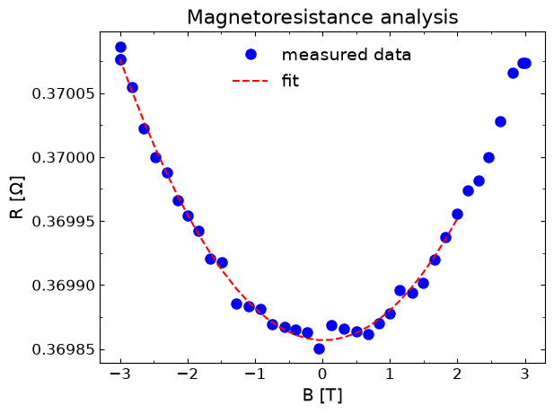

constant: 0.3699 ohm
linear = -7.55E-07 ohm/T
quadratic = 2.42E-05 ohm/T^2
R squared: 0.9942

The only real change in the code is that we created subarrays of our magnetic_field and resistance called magnetic_field_fit and resistance_fit, respectively. This way we can limit the range of data points that go into the fit while still keeping the entire dataset available for plotting. This allows you the ability to overlay the reduced range fitting function over the entire dataset.

17.8.2Initial guesses¶

SciPy’s optimize.curvefit() function by default sets all values initially to 1. We can change this default state by adding the additional argument p0 to the function call. For multiple fitting parameters, p0 accepts a list object with the index order representing the argument order of each parameter in the fitting function. The order starts AFTER the independent variable’s position in the fitting function’s initialization code block, which should be the first argument. So for our magnetoresistance analysis from earlier, p0 would follow the format [constant, linear, quadratic]. The code block below adds this:

# Non-linear fitting example w/ fitting bounds & initial guesses

# -----------------------------------------------------------------------------
# Load data
# -----------------------------------------------------------------------------
iv_data = np.loadtxt("./static/example-data/magnetoresistance-data.csv",
                     delimiter=",",
                     skiprows=2)

magnetic_field = iv_data[:, 0]
resistance = iv_data[:, 1]

# -----------------------------------------------------------------------------
# Data to fit over
# -----------------------------------------------------------------------------

# Data point number
min_index = 7
max_index = 27

# Subset of data to fit over
magnetic_field_fit = magnetic_field[min_index: max_index]
resistance_fit = resistance[min_index: max_index]

# -----------------------------------------------------------------------------
# Least squares analysis
# -----------------------------------------------------------------------------

# Fit the subset! Now includes initial parameters!
popt, pcov = curve_fit(parabolaFunc, magnetic_field_fit, resistance_fit,
                       p0=[0.36, 0, 1E-5])

# Extract parameters
constant = popt[0]
linear = popt[1]
quadratic = popt[2]
constant_err = np.sqrt(pcov[0][0])
linear_err = np.sqrt(pcov[1][1])
quadratic_err = np.sqrt(pcov[2][2])

# Create calculated dataset
resistance_calc = (constant + (linear * magnetic_field_fit)
                  + (quadratic * (magnetic_field_fit**2)))

# R squared
r_squared = rsquared(resistance_fit, resistance_calc)
r_squared = round(r_squared, 4)

# -----------------------------------------------------------------------------
# Plot data
# -----------------------------------------------------------------------------

mr_fig = plt.figure()
mr_fig = mr_fig.add_subplot(1, 1, 1)

# Plot iv data
mr_fig.plot(magnetic_field, resistance,
         label="measured data",
         marker="o",
         markersize=8,
         linestyle="none",
         color="blue")

# Plot fit data
mr_fig.plot(magnetic_field_fit, resistance_calc,
        color="red",
        label="fit",
        linestyle="dashed")

mr_fig.set_title("Magnetoresistance analysis")
mr_fig.set_xlabel("B [T]")
mr_fig.set_ylabel("R [$\\Omega$]")
mr_fig.xaxis.set_minor_locator(tck.AutoMinorLocator(2))
mr_fig.yaxis.set_minor_locator(tck.AutoMinorLocator(2))
mr_fig.legend()


# -----------------------------------------------------------------------------
# Display plot & results
# -----------------------------------------------------------------------------
plt.show()

print(f"constant: {constant:.4f} ohm")
print(f"linear = {linear:.2E} ohm/T")
print(f"quadratic = {quadratic:.2E} ohm/T^2")
print(f"R squared: {r_squared:.4f}")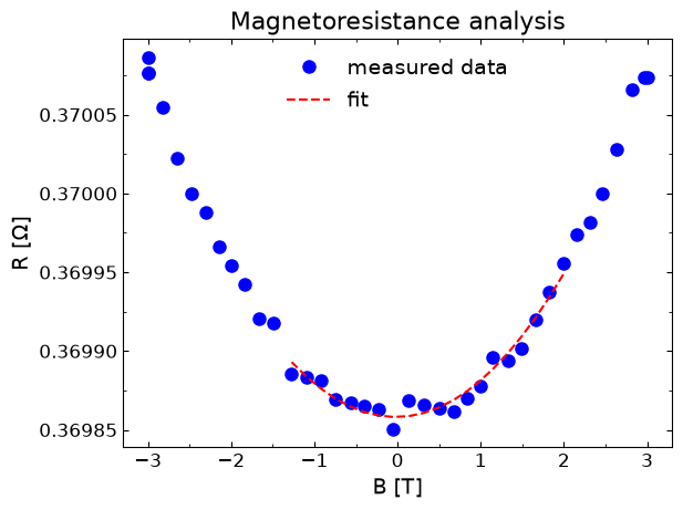

constant: 0.3699 ohm
linear = 9.67E-07 ohm/T
quadratic = 2.23E-05 ohm/T^2
R squared: 0.9582

In this scenario our fitting results with the provided initial guess coverged to our previous results, which is expected given the simplicity of the dataset. Adding initial guesses to your fits are often useful when your data spans orders of magnitudes in values. Since SciPy’s default initial value is 1 for fitting parameters, fitting failures can in these situations. A common error you will see is that your fitting line is flat an you receive the traceback warning:

OptimizeWarning: Covariance of the parameters could not be estimated

What values should you use if you end up in a situation like this? That is where the intuition of the scientist and engineer comes in! Good initial guesses include using expected values from previous measurements, reference data values, and even approximate estimates based on looking at the plotted data (e.g., intercept and slope values). The fitting program will only give you as good results if you give it good starting parts. This is when the learned experience (i.e., wisdom) of a scientist and engineer is vital to solving problems!

17.9Fitting with error bars¶

Including measurement uncertainty on individual data points can also be included in the fitting process. Let’s again revisit our magnetoresistance analysis for this demonstration. We will reuse the majority of the code from this section and update only the necessary lines of code. This time we will use the data file magnetoresistance-data-with-uncertainty.csv. This file is slightly different from the file we used in the previous example, as it also contains estimates on the uncertainty for both the $x$ -value (in this case the magnetic field, $B$ ) and the $y$ -value (the resistance, $R$ ). Even though the data file contains the uncertainty on the $x$ -values, we will not actually use it in the fitting process, as scipy.optimize.curve_fit() only accounts for the uncertainty on the $y$ -values.

Let’s re-run our previous code block with some slight adjustments. See the code below, specifically the lines that have the comment NEW FEATURE HERE! nearby. We further discuss the changes below.

# Fitting with error bars example

# -----------------------------------------------------------------------------
# Load data
# -----------------------------------------------------------------------------
# NEW FEATURE HERE!
data = np.loadtxt("./static/example-data/magnetoresistance-data-with-uncertainty.csv",
                  delimiter =",",
                  skiprows=2)

magnetic_field = data[:,0]
u_magnetic_field = data[:,1]
resistance = data[:,2]
u_resistance = data[:,3]

# -----------------------------------------------------------------------------
# Least squares analysis
# -----------------------------------------------------------------------------

# Fit the subset! (NEW FEATURE HERE!)
popt, pcov = curve_fit(parabolaFunc, magnetic_field, resistance,
                       sigma=u_resistance, absolute_sigma=True)

# Extract parameters
constant = popt[0]
linear = popt[1]
quadratic = popt[2]
constant_err = np.sqrt(pcov[0][0])
linear_err = np.sqrt(pcov[1][1])
quadratic_err = np.sqrt(pcov[2][2])

# Create calculated dataset
resistance_calc = (constant + (linear * magnetic_field)
                  + (quadratic * (magnetic_field**2)))

# R squared
r_squared = rsquared(resistance, resistance_calc)
r_squared = round(r_squared, 4)

# -----------------------------------------------------------------------------
# Plot data
# -----------------------------------------------------------------------------

mr_fig = plt.figure()
mr_fig = mr_fig.add_subplot(1, 1, 1)

# Plot iv data (NEW FEATURE HERE!)
mr_fig.errorbar(magnetic_field, resistance,
                xerr=u_magnetic_field,
                yerr=u_resistance,
                label="measured data",
                marker="o",
                markersize=8,
                linestyle="none",
                color="blue",
                capsize=5)

# Plot fit data
mr_fig.plot(magnetic_field, resistance_calc,
        color="red",
        label="fit",
        linestyle="dashed")

mr_fig.set_title("Magnetoresistance analysis")
mr_fig.set_xlabel("B [T]")
mr_fig.set_ylabel("R [$\\Omega$]")
mr_fig.xaxis.set_minor_locator(tck.AutoMinorLocator(2))
mr_fig.yaxis.set_minor_locator(tck.AutoMinorLocator(2))
mr_fig.legend()


# -----------------------------------------------------------------------------
# Display plot & results
# -----------------------------------------------------------------------------
plt.show()

print(f"constant: {constant:.4f} ohm")
print(f"linear = {linear:.2E} ohm/T")
print(f"quadratic = {quadratic:.2E} ohm/T^2")
print(f"R squared: {r_squared:.4f}")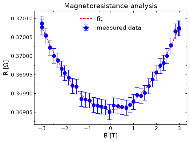

constant: 0.3699 ohm
linear = -2.08E-08 ohm/T
quadratic = 2.46E-05 ohm/T^2
R squared: 0.9946

As you can see in the code, this looks very similar to the previous code but with some tweaks:

After creating the variable data, we now create separate 1D arrays for the uncertainty on $B$ and $R$ called u_magnetic_field and u_resistance, respectively.
The function curve_fit() now contains two additional keyword arguments. The first additional argument is sigma, which represents how much “weight” a particular data point’s uncertainty should influence the overall fit. One common weighting method is called “direct weighting” in which we use the uncertainty of the $y$ -value as the weighting parameter. In this setup, values that have higher uncertainty are weighted more (i.e., prioritized more) in the fit. We do this in our above code block by assigning sigma to u_resistance (i.e., the uncertainty in $R$ ).
The second keyword argument, absolute_sigma=True tells curve_fit() to utilize the actual values provided in sigma in an absolute sense and not in a relative sense. For new users, it is best to set absolute_sigma to True for most situations. Further details on this argument can be found in the online documentation for this function.
We use the Matplotlib Axes method .errorbar() to plot the raw data. This method includes the uncertainty values to each data point as “error bars” to the graph. Overall, .errorbar() works very very similar to .plot() and accepts many of the same keyword arguments. The main difference with .errorbar() is the addition of the keyword arguments xerr and yerr, which represent the error bar values for the $x$ - and $y$ -values, respectively. These are optional arguments, so you do not need to include both arguments when plotting (e.g., sometimes you may want to make a plot with just the $y$ -value error bars).

And with these changes, we now can include the uncertainty of the $y$ -values to our fits!

17.10Final thoughts¶

This lesson explored how Python can be used to complete a task that scientists and engineers often encounter, the fitting of data to a mathematical function. We covered how to fit linear and non-linear data, how to quantify the fit quality through the $R^2$ value, how to add fitting ranges and initial values to the fit, and how to include measurement uncertainty for each data point into the fit. The entire lesson centered around using just the scipy.optimize.curve_fit() function. Overall, the SciPy library is very large and is used in many data processing, optimization, and noise analysis applications. This library, like NumPy and Matplotlib, is an extermely popular external library for scientific and engineering applications. We highly encourage you to take some time to explore what the SciPy library can offer for your programming needs.

17 Data Fitting with SciPy

17.1Lesson goals¶

17.2Overview¶

17.3Installing the SciPy library¶

17.4Importing SciPy for data fitting¶

17.5Linear fitting¶

17.6R2R^2R2 of fit¶

17.7Non-linear curve fitting¶

17.8Other useful fitting options¶

17.8.1Fitting bounds¶

17.8.2Initial guesses¶

17.9Fitting with error bars¶

17.10Final thoughts¶

17.6 $R^2$ of fit¶