1 Getting Started with Python

1.1Lesson goals¶

• Install the Miniforge Python distribution.

• Create a Python virtual environment to handle package compatibility and version control.

• Create a folder on your computer to store this guide’s lessons.

• Install the JupyterLab and Visual Studio Code (VS Code) integrated development environments (IDEs) to assist with Python programming and debugging.

• Learn how to run simply Python code files (PY files) and interactive Python notebook files (IPYNB files).

1.2Overview¶

Python is an excellent programming language to help accelerate your scientific research and engineering projects. It is well suited for many tasks in the scientific domain, such as controlling instruments, analyzing large amounts of data, and automating routine tasks. Python is a free, open-source language with minimalist syntax that makes it easy to get coding quickly, and has a thriving ecosystem of over 600,000 libraries (as of Aug 2026), including standard scientific libraries like NumPy and SciPy. Before we can start programming with Python, we need to install some software. This lesson will will first install Miniforge, which is a common Python distribution. Then we will walk through using Python’s interactive shell via the Miniforge terminal, create and run code files with Visual Studio Code (VS Code), and explore how to use IPython notebook files using JupyterLab.

1.3Installing Miniforge¶

Miniforge is a lightweight Python distribution available for all operating systems. Unlike larger distributions, it provides a minimal pre-configured setup that is use the free and has access to a community-driven library repository (the conda-forge repository), allowing you to install exactly the tools you need without bloat. In this guide, we will be using the latest version of Miniforge. Below are instructions for installing Miniforge on Windows or Mac:

• Installing Miniforge on Windows

• Installing Miniforge on macOS

1.4Launching the Miniforge Prompt¶

After installing Miniforge, you will need to launch the Miniforge Prompt to access conda, which is a popular package and environment manager. The Miniforge Prompt is a specialized terminal that is pre-configured to run conda and its commands. A terminal, also known as a console or command line, is an interface that allows you to type commands directly to your computer’s operating system. When you open the prompt, you will know it is set up correctly if you see a (base) prefix at the start of the line. This indicates that conda is active and you are currently in the default base environment. Starting Miniforge for Windows and macOS are detailed below.

1.4.1Starting Miniforge in Windows¶

In Windows, go to the “Start Menu” and type Miniforge Prompt:

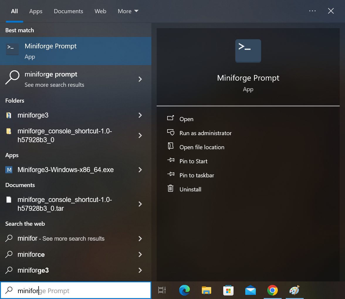
This opens a terminal window with the (base) environment activated. You should see a prompt like:

(base) C:\Users\YourName>

1.4.2Starting Miniforge in macOS¶

On macOS, go to Spotlight, type in Terminal, and click the “Terminal” application. The Miniforge installer configures your terminal to activate conda automatically, so you should see (base) at the beginning of your prompt:

(base) yourname@mac ~ %

1.4.3Note for Anaconda users¶

Repositories in conda are referred to as channels. This guide will be using the conda-forge package repository since it is the default channel for Miniforge. The conda-forge channel contains all of the necessary Python libraries we will need for this guide and they are updated frequently.

Anaconda is an very popular Python distribution and there is a good chance you may have used this before if you have tried out Python. If you have Anaconda installed and do not want to remove its channel, you will need to manually specify the conda-forge channel every time you install a new package. You can do this by adding -c conda-forge to your installation commands (we will see how to install packages very soon):

conda install -c conda-forge <package_name>

If you have recently uninstalled Anaconda, its channel repository configuration may still be lingering on your computer. To ensure we are only using conda-forge for this guide, we can remove the Anaconda defaults channel from your conda configuration. First, check your current channel in conda by typing in the following command into the Miniforge Prompt and pressing ENTER:

conda config --show channels

If you see defaults in the output of the command, we need to remove that channel. To remove it, type the following command and press ENTER:

conda config --remove channels defaults

1.5Creating virtual environments¶

Virtual environments allow you to setup different Python libraries for different projects, which helps avoid version conflicts between libraries used for these projects. It is recommended to create a virtual environment for each Python project rather than installing everything into the default base environment. Let’s create a new virtual environment named mats5000 to be used in this guide. To do this, first type the following in the Miniforge Prompt and press ENTER:

conda create -n mats5000

You will be asked to confirm the installation. Type y and press ENTER to proceed. Once the environment is created you can activate your new environment by typing:

conda activate mats5000

Notice on the left side of your terminal the prompt changes from (base) to (mats5000), which confirms that we are now working in the mats5000 environment. Any Python libraries you install with conda install will then only be installed in this environment.

If you forget the names of your environment, you can always list them all out with the conda env list command:

conda env list

# conda environments:
#
# * -> active
# + -> frozen
base                     C:\Users\myuser\miniforge3
mats5000              *  C:\Users\myuser\miniforge3\envs\mats5000

1.6Installing packages¶

Right now the mats5000 environment is completely empty. We can verify this using the conda list command, which displays all the packages and libraries currently installed in the currently active environment:

conda list

# packages in environment at /Users/myuser/miniforge3/envs/mats5000:
#
# Name                    Version                   Build  Channel

If you look closely at the output of that command, you will see a file path pointing to a specific folder on your computer (/Users/myuser/miniforge3/envs/mats5000). This is how conda manages different environments behind the scenes, each virtual environment simply gets its own folder.

The output also shows that nothing is currently installed in the virtual environment. Let’s fix this by installing the base Python package. The Python library, just like many other libraries that we will use later in this guide, comes in many different versions. With conda we can search the conda-forge channel to see all available versions of a package using the conda search command:

conda search -c conda-forge python

Loading channels: done
# Name                       Version           Build  Channel
...
python                        3.14.6 h7c1dbca_1_cp314t  conda-forge
python                        3.14.6 hb4b0029_2_cp314t  conda-forge
python                        3.14.7 h53f6dd8_100_cp314  conda-forge
python                        3.14.7 hb4b0029_0_cp314t  conda-forge

We can see a long list of many different versions of Python. New versions of Python are released periodically, and older versions are eventually retired, and so it is good practice to install a recent, stable version. The latest version as of August 2026 is 3.14, but for our guide, we will use 3.13. With conda, we can specify the specific version with a single equals sign = after the package name followed by the version number. The prompt below installs Python version 3.13 to our environment:

conda install python=3.13

Conda will take some time to evaluate what needs to be downloaded, and then should prompt you to confirm. Type y (for yes) and press ENTER to complete the installation. Python should now start installing on your computer.

1.7Running the Python interactive shell¶

We can use Python’s shell program (i.e., an application that interprets and executes code) to enter in commands and getting results quickly. Since the shell will be reading commands directly typed by us, we call this an interactive shell.

First, activate the mats5000 environment in your Miniforge Prompt:

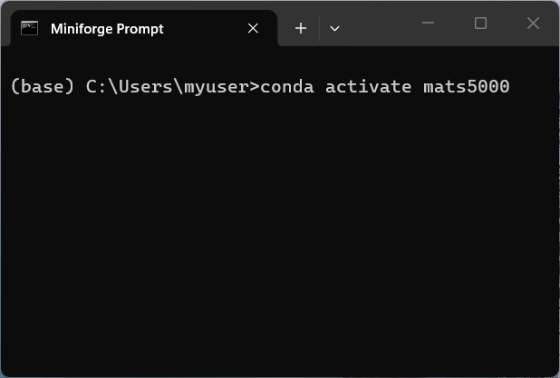
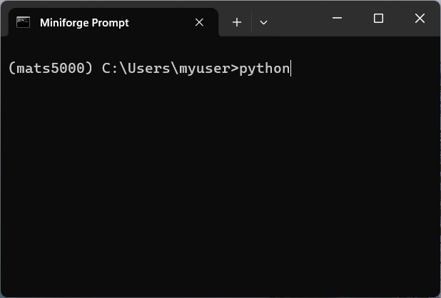
Then type python and press ENTER. The image below shows this step using Miniforge Prompt in Windows:

Now you are in the Python interactive shell! We can start typing in commands to use Python. For example, we can use the shell as a calculator. Let us answer the age-old question: What is one plus four? Type in 1+4 in the prompt (after the >>>) and press ENTER on the keyboard to see the answer:

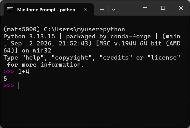
You can see we got an output right away, 5, which settles that question. This demonstrates how the interactive shell “reads” an input using the Python interpreter, “evaluates” the result, “prints” out an output, and the “loops” back to reading. This programming pattern is often referred to as REPL. The interactive shell is a great way to quickly get an answer to something using Python, it simply requires typing in some commands and pressing ENTER to get a result.

The downside of the interactive shell is that you have to retype all the commands each time you open it up. In the next section, we will explore how to store code in an external file and then have the Python interpreter parse that file.

1.8Running Python code files in VS Code¶

Python code files are simply text files that contain Python commands and have a filename that ends with the file extension .py. We could use simple text editors like Notepad on Windows or TextEdit on Mac to create and edit Python files. However, programmers like to be efficient (or lazy), and want to have additional features on top of the text editor to help them code, such as built-in error checking and automatic tab completion. Therefore, some programmers have replaced simple text editors with “integrated development environments”, or IDEs, which have features to help them code quickly and correctly. We will be using a popular IDE called Visual Studio Code (or simply “VS Code”) by Microsoft.

Let’s try running Python code files using VS Code. The steps below detail how to set up our computer to get things running.

1.8.1Create a working folder¶

We recommend creating a dedicated folder as a workspace to keep files organized as you work through this guide. Below are two short guides on how to create a folder called mats5000 in your Document folder for both Windows and macOS.

• Creating a folder on Windows

• Creating a folder on MacOS

1.8.2Install and configure VSCode¶

The next step is to install VS Code on your computer. Below are installation guides for both Windows and macOS:

• Install VS Code on Windows

• Install VS Code on macOS

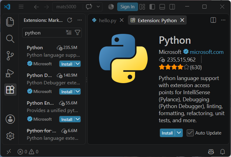
On first launch you may see a welcome screen prompting for an account, you do not need to create an account to use VS Code. Next, we need to install the Python extension for VS Code. Open the “Extensions” view by clicking the icon (four blocks) on the left sidebar. Search for “Python”, locate the extension published by Microsoft, and click “Install”.

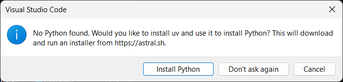
If the following prompt appears stating “No Python found”, you may disregard it since Miniforge is already installed. Select “Don’t ask again” or “Cancel”.

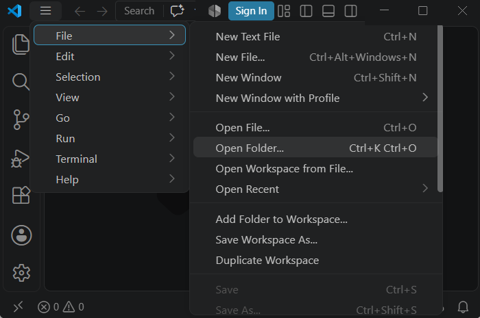
Now let’s open our Documents/mats5000 folder. Go to “File” in the top menubar and select “Open Folder”.

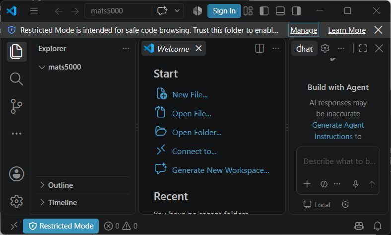
Navigate to your Documents/mats5000 folder, and click “Select Folder”. The first time you open a folder you will be prompted if you would like to “Trust” the folder. Click on “Manage” on the top.

Then scroll down and click on the “Trust” button:

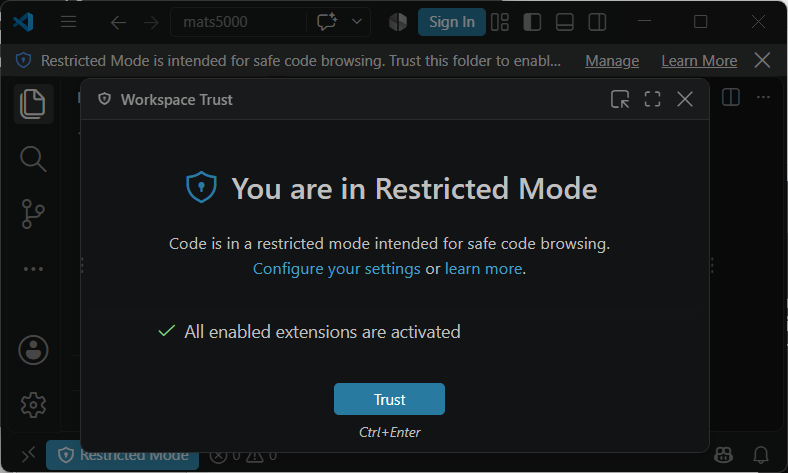
You will now have the ability to read and write to this folder.

1.8.3Download hello.py¶

Download the hello.py demo file and save it to your Documents/mats5000 folder. You should now see “hello.py” in the left sidebar, which shows the contents of the “mats5000” folder.

In order to run Python files in VSCode, we need to configure a Python interpreter for the workspace. We will point VS Code at the mats5000 virtual environment we have already created. While you have “hello.py” selected, click on the “Select Python Interpreter” button on the bottom right corner:

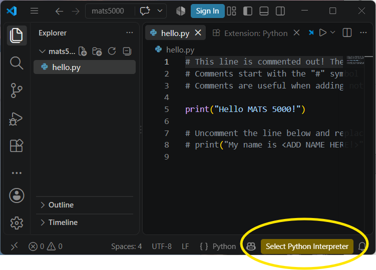
This will prompt a top dropdown where we can point VS Code to the Python environment we want to use. Select “mats5000” from the top dropdown:

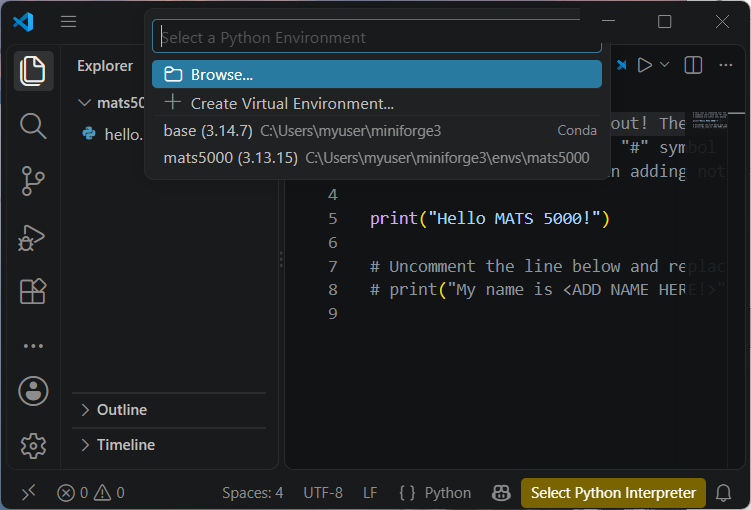
The VS Code workspace is now configured with our Python interpreter, and we can now run Python files in the IDE. Now click the “Play” button in the top right corner.

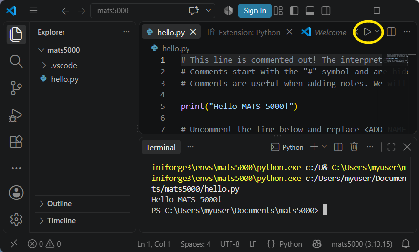
The IDE will open a new terminal, activate the configured Python environment, and run the Python file! You can see the output from the Python code prints Hello MATS 5000! to the terminal.

1.9Running JupyterLab notebooks¶

Up to this point, we have showed two different ways to execute Python code, running commands directly in the shell and creating and running .py files. Each way has its own advantages and disadvantages. Fortunately, both JupyterLab and VS Code IDEs provide an interactive computing environment that combines the interactivity of the Python shell with the long form coding format of Python files through the use of IPython notebooks (a.k.a. Jupyter notebooks).

Let’s demonstrate how an IPython notebook file works using the JupyterLab IDE. We first need to install JupyterLab to our Python environment. If not done so already, open up a Miniforge Prompt terminal session and activate the mats5000 environment. Now type in the the following command which will install JupyterLab and a specific IPython kernel library we will use in this guide:

conda install jupyterlab ipykernel=6.31

Then launch JupyterLab by typing the following and pressing ENTER:

jupyter lab

JupyterLab should by default open a new tab in your web browser with localhost:8888/lab in the address bar:

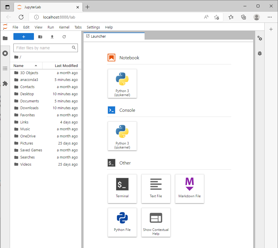
This is the JupyterLab workspace. On the left is a sidebar containing the file manager. The file manager opens up in the current folder space of the Miniforge Prompt (usually your user profile folder). Next to the sidebar is the main editor window. This is where IPython notebooks and files are displayed and edited. By default, the main editor window has a single tab open showing various JupyterLab “Launchers”. On the Launcher tab, under “Notebook”, click the “Python 3 (ipykernel)” launcher to open a new Jupyter notebook. The image below has a red circle around the Jupyter notebook launcher:

We can now edit our first Jupyter notebook! Below is an image of a blank IPython notebook file:

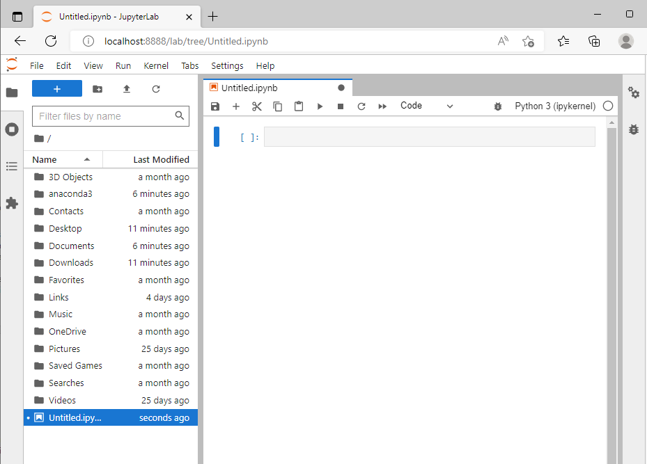
In the sidebar file manager we can see a new file is now highlighted “Untitled.ipynb”. This is our new Jupyter notebook file that we have created and are now editing. The .ipynb file extension denotes that it is a Jupyter notebook file (i.e., an IPython notebook file).

The main editor window now displays our Jupyter notebook. Select the grey rectangle in the main editor window, which is called a code cell. Once you have selected the cell, your cursor should start blinking. Type in 1+4, press SHIFT and ENTER key at the same time (SHIFT + ENTER), and see what happens:

You have just run the code in that code cell! Now les us explore and explain the notebook environment some more:

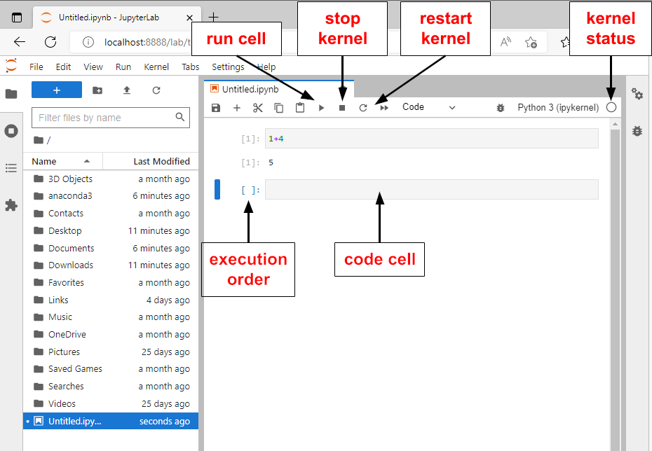
1. Code cell: The gray area is where you type Python code.

2. Execution order: The brackets next to the code cell denotes the order the cell was run. This is explained below.

3. Run cell: This button executes the current cell, the same action as pressing SHIFT + ENTER

4. Stop kernel: This button interrupts the background kernel process.

5. Restart kernel: This button restarts the background kernel process. This is explained further down below.

6. Kernel status: This circle icon denotes if the kernel is executing code or in an idle state. When empty, it is idle, when full, it is running

There are a couple of concepts that are useful to understand about the notebook environment: the kernel, the execution order of commands, and notebook management.

1.9.1The kernel¶

The kernel is a background process that executes each code cell one at a time. Like the Python interactive shell, the kernel reads the code that you’ve typed in, evaluates it, and prints out the output. The kernel starts up once you’ve opened a notebook.

The status of the kernel is displayed in the top right of the browser. When you are executing a code cell, and the kernel is processing the commands, the circle next to “Python 3 (ipykernel)” should be filled in. When execution is complete, the circle should be empty which denotes the kernel is idle.

1.9.1.1Kernel interruption¶

Sometimes, or more likely often, we make mistakes when coding. Perhaps we have started executing a code cell that has a mistake in it, and you’d like to stop the kernel. There are two ways to interrupt the kernel from running. One option is to click the square stop button to interrupt the kernel and halt the current execution. The image below shows the location of this button:

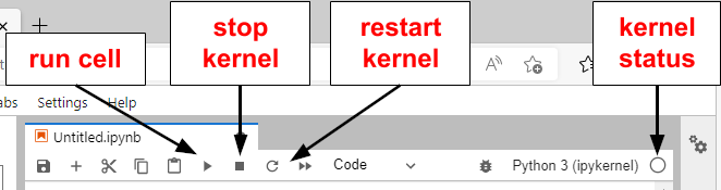
Alternatively, you can click the restart kernel button. This will first interrupt the kernel and then restart the entire kernel session. Clearing the kernel session means the variables that were assigned will be cleared, every code cell that has been run will be removed from memory. Code cells will have to be executed again from the beginning. Restarting the kernel is useful if you want to start your notebook again with a fresh state.

1.9.2Execution order¶

As we evaluate code cells we are changing the state of the ipython notebook. The order in which we evaluate code cells is the called the execution order. The execution order is denoted by the number in the brackets to the left of the code cell. If you were to press SHIFT + ENTER from start to end of a notebook, the kernel would evaluate all the code cells in the order they are displayed. However, you do not have to evaluate code cells in order, and in fact you can run code cells in any order you want. This is important to keep in mind to understand the output of an IPython notebook.

Here is a concrete example: How is it that print(a) outputs 16 when in the previous cell we had just assigned a = 4 + 1?

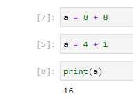
The answer is in the execution order of the cells. From the number within the brackets, the execution order, it is clear the top cell was run ([7]), and then right away the bottom cell was run ([8]). That is why the final output can be 16 instead of 5. At a glance this can look out of place, so it is important to note the execution number in the brackets to follow the output in a notebook.

1.9.3Notebook management¶

Finally, a few miscellaneous notes regarding Jupyter notebook management. You can rename any Jupyter notebook by right-clicking the file name and selecting “Rename” from the context menu.

JupyterLab will autosave the Jupyter notebook every two minutes, but you can also manually save by going to the menu and clicking File -> “Save Notebook”, or using the shortcut CTRL+S on Windows or CMD+S on Mac.

1.10Final thoughts¶

1. Installed Miniforge

2. Launched the Miniforge Prompt to access conda and Python

3. Created and managed virtual environments with conda

4. Launched the Python interactive shell

5. Installed and launched JupyterLab to run notebooks